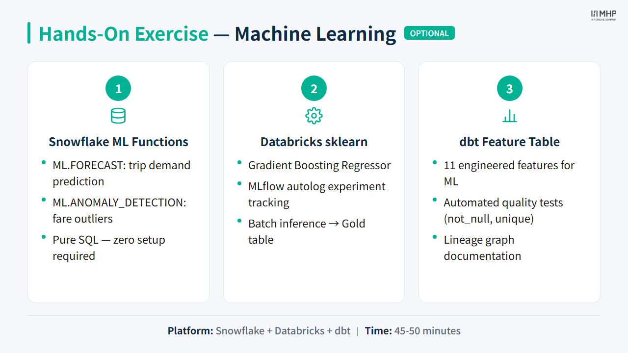
Module 9: Machine Learning (Optional)

Optional · Tip prediction on NYC Taxi Silver

Duration: 90 min — Animation (3) · Think & Discuss (8) · Theory (20) · Quiz (3) · Practice (56)

1. Animation

Story animation — mod-09-ml.mp4

Live delivery: your trainer narrates from the Module 9 section of the animation voiceover script if the MP4 is not available.

When MP4 is ready, add to media/modules/mod-09-ml.mp4 and re-run scripts/_scaffold_generate.py for automatic embed.

2. Think & Discuss

Situation: Marcus wants tip prediction on credit-card trips only. Lab uses existing NYC Taxi Silver from Modules 2–3.

Prompts:

• Why must total_amount not be a feature when predicting tip_amount?
• Why train on credit-card trips only?
• Who builds the feature table vs who trains the model?

3. Theory

Slide 37

Machine Learning — Predictive ML Patterns

WarningNot Module 6 again

Module 6 was Cortex LLM assistants. This module is predictive ML — sklearn, Snowpark ML, and ML.FORECAST.

Note

Snowflake ML Functions are distinct from the Cortex LLM features covered in Module 6.

NotePrerequisites

Modules 2–3 required · Module 4 recommended (dbt feature table track). Deliver after Module 8 when following YellowLine NYC Phase 2 story.

NoteSnowflake forecasting APIs

Labs use TABLE(ML.FORECAST(...)) as a table function. Production may use CREATE SNOWFLAKE.ML.FORECAST for persistent models — Snowflake forecasting docs.

Note3.1 Optional Module

This module is delivered after the main workshop or as a standalone advanced session. It builds directly on the Silver enriched table from Modules 2 and 3 — no new data, just a new use of the data you already built.

Duration: 90 minutes

3.2 Use Case: Predict NYC Taxi Tip Amount

Problem: Given trip characteristics at the time of dropoff, predict how much tip a passenger will leave.

This is a regression problem — we predict a continuous value (tip_amount in USD), not a category.

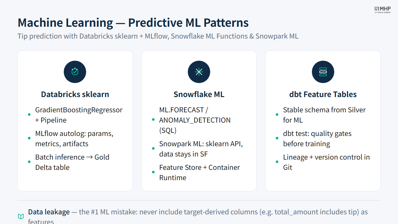
Why tip prediction? - Target variable tip_amount is already in the Silver table — no new data collection - Features are fully engineered: trip distance, time of day, borough, fare amount - Results are interpretable: trainees understand what makes a higher tip - Well-known benchmark — easy to find reference RMSE values online

---

3.3 Theory: Where ML Fits in the Data Lifecycle

flowchart LR
    A["Raw Data\nADLS2"] --> B["Bronze\nIngest"]
    B --> C["Silver\nClean + Enrich"]
    C --> D["Gold\nKPI Aggregates"]
    C --> E["ML Feature Table\ndbt"]
    E --> F["Model Training\nDatabricks / Snowflake"]
    F --> G["ML Predictions\nGold Table"]
    D --> H["Power BI\nDashboard"]
    G --> H

    style A fill:#0057b8,color:#fff,stroke:#003d82
    style B fill:#475569,color:#fff,stroke:#334155
    style C fill:#0369a1,color:#fff,stroke:#075985
    style D fill:#01065c,color:#fff,stroke:#000940
    style E fill:#6d28d9,color:#fff,stroke:#5b21b6
    style F fill:#6d28d9,color:#fff,stroke:#5b21b6
    style G fill:#4c1d95,color:#fff,stroke:#3b0764
    style H fill:#107c10,color:#fff,stroke:#0a5c0a

Data engineers build up to the feature table. Data scientists train and deploy models. In this module, we play both roles.

Data leakage: the most common ML mistake

Leakage means including information in your features that wouldn’t be available at prediction time, or that mathematically encodes the answer.

Warning⚠️ What must NOT be a feature here

Column	Why it’s leakage
total_amount	= fare + tip + surcharges — directly includes the target
tip_percentage	= tip / fare × 100 — mathematically derived from target
payment_type (if using all)	Cash is always 0 tip — model just learns “cash = no tip”, not real signal

Safe features: trip_distance, fare_amount, pickup_hour, day_of_week, pickup_borough, dropoff_borough, passenger_count, time_of_day

Why credit card trips only?

Cash payments always record tip_amount = 0 — the passenger pays in cash and no tip is entered digitally. If we include cash trips, the model learns “cash → 0 tip”, polluting the real relationship between trip features and tipping behaviour.

Filter: WHERE payment_type_desc = 'Credit Card'

---

3.4 Part 1: Databricks — sklearn + MLflow

Databricks Runtime ML includes sklearn, XGBoost, LightGBM, and MLflow out of the box.

The training pattern

import mlflow
import mlflow.sklearn
from sklearn.ensemble import GradientBoostingRegressor
from sklearn.pipeline import Pipeline

# Load from Silver Delta table
df_pd = (
    spark.table(f"{catalog}.{silver_schema}.silver_nyc_taxi_enriched")
    .filter(col("payment_type_desc") == "Credit Card")
    .sample(fraction=0.10, seed=42)
    .toPandas()                              # Spark → Pandas for sklearn
)

# Train with MLflow autolog — captures everything automatically
mlflow.sklearn.autolog(log_input_examples=True)

with mlflow.start_run(run_name=f"tip_prediction_{ATTENDEE_ID}"):
    model.fit(X_train, y_train)
    mlflow.log_metrics({"rmse": rmse, "mae": mae, "r2": r2})

Key concepts

train_test_split: Hold out 20% of data to evaluate how well the model generalises to unseen trips.

GradientBoostingRegressor: An ensemble of decision trees — each tree corrects the errors of the previous one. Strong default model for tabular data.

mlflow.sklearn.autolog(): One line captures all hyperparameters, train/test metrics, and the model artifact. View results in Experiments sidebar.

Batch inference: After training, score the full Silver table and write {attendee_id}_gold.ml_tip_predictions — a Gold table combining actual and predicted tips for Power BI.

NoteMosaic AI Model Serving (production pattern)

In this workshop, we use batch inference (score the full Silver table, write to Gold). Production deployments typically use Mosaic AI Model Serving — a managed REST endpoint that serves MLflow-registered models with auto-scaling.

Validate with cross-validation, not just one split

A single train_test_split can produce misleading metrics if the random split happens to favor easy or hard examples. For production models, use k-fold cross-validation (cross_val_score with k=5) to get a more robust estimate of model performance. In this workshop, a single split is sufficient to learn the workflow — but never ship a model to production based on one random split alone.

Feature importance

gbr = model.named_steps["model"]
importance_df = pd.DataFrame({
    "feature": feature_names,
    "importance": gbr.feature_importances_
}).sort_values("importance", ascending=False)

Tip3.5 Discussion question

Which feature ranks highest? Is fare_amount the dominant predictor — and does that make intuitive sense? Is it borderline leakage?

Stretch: Databricks AutoML

AutoML tries XGBoost, LightGBM, RandomForest, and others automatically, then presents the winning notebook for inspection.

UI path: Experiments → Create AutoML Experiment → Regression → select Silver enriched table → target tip_amount → Start

---

3.6 Part 2: Snowflake — Two Approaches

Approach A: Snowflake ML Functions (SQL only)

Snowflake ML Functions are built-in Snowflake TABLE functions — ML as a SQL clause.

-- Predict future trip demand per borough (next 24 hours)
SELECT * FROM TABLE(
    ML.FORECAST(
        INPUT_DATA        => SYSTEM$REFERENCE('TABLE', 'GOLD_TRIPS_BY_HOUR'),
        TIMESTAMP_COLNAME => 'PICKUP_HOUR_TS',
        TARGET_COLNAME    => 'TOTAL_TRIPS',
        SERIES_COLNAME    => 'PICKUP_BOROUGH',
        CONFIG_OBJECT     => {'prediction_interval': 24}
    )
);

-- Detect hours with anomalous average fares
SELECT * FROM TABLE(
    ML.ANOMALY_DETECTION(
        INPUT_DATA        => SYSTEM$REFERENCE('VIEW', 'V_HOURLY_FARES'),
        TIMESTAMP_COLNAME => 'FARE_HOUR',
        TARGET_COLNAME    => 'AVG_FARE',
        SERIES_COLNAME    => 'PICKUP_BOROUGH',
        LABEL_COLNAME     => NULL   -- unsupervised
    )
);

What Snowflake ML Functions return:

Function	Output columns
ML.FORECAST	SERIES, TS (future timestamp), FORECAST, LOWER_BOUND, UPPER_BOUND
ML.ANOMALY_DETECTION	SERIES, TS, Y (actual), ANOMALY (bool), ANOMALY_SCORE

No training, no model management, no Python — results appear in one SQL statement.

Approach B: Snowpark ML (Python)

Snowpark ML has an sklearn-compatible API where all training runs on Snowflake’s compute.

from snowflake.ml.modeling.ensemble import GradientBoostingRegressor

# Note: identical class name and hyperparameters as sklearn
model = GradientBoostingRegressor(
    input_cols  = FEATURE_COLS,
    label_cols  = ["TIP_AMOUNT"],
    output_cols = ["PREDICTED_TIP"],
    n_estimators = 200,
    learning_rate = 0.05,
)

model.fit(df_snowpark)          # df is a Snowpark DataFrame — data stays in Snowflake
df_predictions = model.predict(df_test)

Critical difference from Databricks:

	Databricks (sklearn)	Snowflake (Snowpark ML)
Data flow	.toPandas() → driver → sklearn	Stays in Snowflake compute
Training location	Driver node (or distributed)	Snowflake warehouse
Data movement	Yes — to Python process	None
API	from sklearn.ensemble import ...	from snowflake.ml.modeling.ensemble import ...

---

3.7 Part 3: dbt — Feature Engineering & Quality Gates

dbt does not train models. It defines the canonical feature table that both training pipelines consume.

-- ml/dbt/models/ml_features_tip_prediction.sql
{{ config(materialized='table', tags=['ml', 'features']) }}

SELECT
    trip_distance, fare_amount, passenger_count,
    pickup_hour, pickup_day_of_week,
    CAST(is_weekend AS INTEGER) AS is_weekend,
    time_of_day, pickup_borough, dropoff_borough,
    tip_amount AS target_tip_amount
FROM {{ ref('silver_nyc_taxi_enriched') }}
WHERE payment_type_desc = 'Credit Card'
  AND tip_amount >= 0
  AND fare_amount > 0

Run it:

dbt run  --select ml_features_tip_prediction
dbt test --select ml_features_tip_prediction

Why this matters for MLOps

flowchart LR
    S["silver_nyc_taxi_enriched"] --> F["ml_features_tip_prediction\ndbt table"]
    F --> DB["Databricks\nsklearn training"]
    F --> SF["Snowflake\nSnowpark ML training"]

    style S fill:#0369a1,color:#fff,stroke:#075985
    style F fill:#6d28d9,color:#fff,stroke:#5b21b6
    style DB fill:#01065c,color:#fff,stroke:#000940
    style SF fill:#01065c,color:#fff,stroke:#000940

• Stability: Data scientists consume a named table with a stable schema. Silver schema changes don’t silently break training notebooks.
• Quality gates: dbt test checks every feature column before the model trains. If tip_amount has nulls, the test fails — poisoned data never reaches training.
• Lineage: dbt docs shows the full path from raw data to features. When a model’s accuracy drops, you can trace back to which upstream table changed.
• Version control: Feature logic is a SQL file in Git — reviewable, diffable, tagged to model versions.

NoteDatabricks Feature Store

Databricks also offers Unity Catalog feature tables (formerly Feature Store) for point-in-time correct feature lookups. For this workshop’s scope, dbt tables are sufficient.

---

3.8 Full Comparison: ML across all three tools

Aspect	Databricks (sklearn)	Databricks AutoML	Snowflake ML Functions	Snowflake Snowpark ML	dbt
What it does	Custom model training	Automated training + code generation	4 managed ML functions (no model code needed)	Custom training on Snowflake compute	Feature table definition only
Interface	Python	Databricks UI + generated Python	SQL only	Python (snowflake-ml-python) + SQL	SQL
Data location during training	Driver (via .toPandas()); use Spark UDFs or SPCS for larger datasets	Driver	Stays in Snowflake	Stays in Snowflake (Snowpark DataFrame; Container Runtime for distributed scale)	N/A
Algorithms	Any sklearn / PyTorch / TF / XGBoost	sklearn family	FORECAST, ANOMALY_DETECTION, CLASSIFICATION, TOP_INSIGHTS only (no custom algorithms)	sklearn, XGBoost, LightGBM, PyTorch, CatBoost, Prophet + more	N/A
Model tracking	MLflow (manual or autolog)	MLflow (auto)	Not in Model Registry — stored as SQL DDL schema-level objects	Snowflake Model Registry (snowflake-ml-python ≥ 1.5.0)	N/A
Inference	Batch → Delta Gold table	Batch → Delta Gold table	model_name!PREDICT() or CALL model!FORECAST() in SQL (runs in warehouse)	mv.run() (Python) or SQL call in warehouse	N/A
Effort	Medium	Low	Very low	Medium	Low
Explainability	Feature importance + SHAP	SHAP (generated notebook)	CLASSIFICATION: SHOW_FEATURE_IMPORTANCE; FORECAST/ANOMALY_DETECTION: none	SHAP via mv.explain() (GA in current Snowflake releases)	N/A
Custom algorithms	✅ Any	Partial (sklearn family)	❌ (fixed function types only)	✅ Any Python ML library (warehouse or Snowpark Container Services)	N/A
Python required	Yes	No (UI-driven)	No	Yes	No
Best for	Maximum algorithm flexibility, deep MLflow tracking	Fast baseline for non-ML engineers	No-code ML for analysts; time-series forecasting & classification	Python teams whose data is already in Snowflake	Feature governance and quality gates

Tip3.9 When to use which?

• Snowflake ML Functions first — if ML.FORECAST, ML.ANOMALY_DETECTION, ML.CLASSIFICATION, or ML.TOP_INSIGHTS covers your use case, this is the lowest-friction path: pure SQL, no model code, no infrastructure. Note these models are not stored in the Snowflake Model Registry — they are schema-level DDL objects managed via SQL commands.
• Snowpark ML — when you need custom algorithms and all data is already in Snowflake. No .toPandas() overhead.
• Databricks sklearn/AutoML — when you need full algorithm flexibility, deep MLflow tracking, or you already run your compute on Databricks.
• dbt — always, to define and test feature tables, regardless of which training platform you use.

3.10 Key Takeaways

• ML fits after Silver — data engineers build the feature table; data scientists (or the same person) train the model
• Data leakage is the #1 ML mistake: total_amount includes the target, cash trips encode “no tip” — both destroy model validity
• Databricks offers maximum flexibility (any sklearn algorithm, MLflow tracking, AutoML) but requires .toPandas() data movement
• Snowflake ML Functions cover most business ML needs with zero Python — pure SQL forecasting, anomaly detection, classification
• Snowpark ML trains on Snowflake compute without data movement — ideal when all data is already in Snowflake
• dbt governs the feature table — tested, versioned, lineage-tracked features prevent silent model breakage
• Cross-validation (not a single train/test split) is the production standard for robust model evaluation

4. Quiz

Quiz: Module 9 — Machine Learning Quiz

Scan QR to open quiz

Before moving on, make sure you can answer:

1. Why must total_amount never be used as a feature when predicting tip_amount?
2. What is the key difference between Databricks sklearn training (.toPandas()) and Snowpark ML training (data stays in Snowflake)?
3. When would you choose Snowflake ML Functions over Snowpark ML or Databricks sklearn?

5. Practice

Slide 38

Hands-On Exercise — Machine Learning

Hands-on lab

• Exercise: Machine Learning

After the exercise, your trainer facilitates a 10-minute comparison of Databricks, Snowflake Cortex, Snowpark ML, and dbt feature tables (lowest effort, most flexibility, SQL-only team).

Priya / Power BI: Predicted vs actual tip view in Power BI — batch scoring table from Gold.

Next module

End of YellowLine NYC Phase 2 — revisit Module 7: Comparison & Wrap-up tool choices with streaming/ML constraints.

---

Official Documentation

• Snowflake ML forecasting
• Snowflake Model Registry
• MLflow on Databricks
• Snowpark ML